An R package for generating and simulating in silico biological systems.

Introduction
Creating an in silico system
Creating an in silico population
Simulating the system
- Plotting the simulation
- The stochastic model
  - The species
  - The reactions
Generating RNA-seq-like data
Appendix
- Parameters for in silico system generation
- Parameters for in silico individuals generation

Introduction

The sismonr package aims at simulating random in silico biological systems, containing genes linked through networks of regulatory interactions. The regulatory interactions can be of different type, i.e. we account for regulation of transcription, translation, RNA decay, protein decay and protein post-translational modification. sismonr then simulates the stochastic expression profiles of the different genes in these systems over time for different in silico individuals, where the individuals are distinguised by the genetic mutations they carry for each gene, affecting the properties of the genes. The user has control over the different parameters used in the generation of the genes, the regulatory network and the individuals.

Here we describe how to use the sismonr package. The code used throughout this documentation as well as the created variables saved as .RData objects are available here.

Installation

The sismonr package depends on the programming language Julia. It is preferable to install Julia on your computer before installing sismonr.

Installing Julia

To install Julia, go to https://julialang.org/downloads/ and follow the instructions. The sismonr package currently works with version >= 1.0.

Please make sure to include the Julia executable in your environmental variable PATH. Linux users can use the following command in the terminal:

sudo ln -s path_to_julia_folder/bin/julia /usr/local/bin/julia

to create a symbolic link to julia inside the /usr/local/bin folder.

Windows users can open the Control Panel and go to System > Advanced system settings > Environment variables. Select the PATH variable, click on Edit > New and copy-paste the path path_to_julia_folder/bin.

Installing sismonr

sismonr is available on the CRAN. You can install sismonr from R or Rstudio using the following commands:

install.packages("sismonr")

Alternatively, to download the latest development version, you can use:

library(devtools)
install_github("oliviaAB/sismonr")

A first note

The sismonr package uses the programming language Julia to speed up computations for some of the functions. Note that the user doesn’t need to have any knowledge of Julia to use sismonr, all calls to Julia are handled internally. When starting a new R session, the first call to any sismonr function using Julia will therefore take a few seconds longer than usual (and print a blank line), as sismonr is starting a new Julia process to run the underlying Julia commands.

Abbreviations

Here are the notations used throughout the sismonr package:

Abbreviations	Meaning
TC	Transcription
TL	Translation
RD	RNA decay
PD	Protein decay
PTM	Post-translational modification

PC	Protein-coding
NC	Noncoding

Pr	Promoter binding site
RBS	RNA binding site
R	RNA
P	Protein
Pm	Modified protein
C	Regulatory complex

Creating an in silico system

The first step is to generate an in silico system. An in silico system is composed of a set of genes, and a gene regulatory network or GRN describing the different regulatory interactions occuring between the genes. The system is created by a call to the function createInSilicoSystem. The user can control different aspects of the system with the arguments passed to the function. For example:

mysystem = createInSilicoSystem(G = 10, PC.p = 0.7, ploidy = 2)

generates an in silico system with 10 genes, and during the generation process each gene has a probability of 0.7 to be a protein-coding gene (as opposed to noncoding gene). The ploidy arguments controls how many copies of each gene will be present in the system. Here ploidy = 2 generates a diploid system. If not specified, the ploidy parameter will automatically be set to 2. The system returned by the function is an object of class insilicosystem, i.e. a list whose different attributes are presented below.

The list of genes

The different genes constituting the system are stored in a data-frame, and can be accessed with:

> mysystem$genes

   id coding TargetReaction PTMform ActiveForm       TCrate     TLrate       RDrate       PDrate
 1     NC            PTM       0         R1 0.0022650092 0.00000000 0.0006022248 0.000000e+00
 2     PC             RD       0         P2 0.0011610575 1.45493135 0.0012704290 5.241792e-04
 3     PC             TL       0         P3 0.0008440692 0.07610997 0.0005346026 4.659461e-04
 4     PC             MR       0         P4 0.0018660167 0.02094220 0.0005450206 9.495481e-05
 5     PC             TC       0         P5 0.0013195158 0.08482105 0.0015738163 3.724944e-04
 6     NC             TL       0         R6 0.0017867835 0.00000000 0.0009361317 0.000000e+00
 7     PC             TC       1        Pm7 0.0050424625 0.08673830 0.0003888850 9.668181e-04
 8     PC             TC       0         P8 0.0040488925 0.52078680 0.0008828149 2.566280e-04
 9     NC             TL       0         R9 0.0008180618 0.00000000 0.0007097201 0.000000e+00
10     NC             TC       0        R10 0.0034226576 0.00000000 0.0003839845 0.000000e+00

Each gene is labeled with an ID (column id) and possesses the following parameters:

coding: gives the coding status of the gene, i.e. describes if the gene is protein-coding (coding = "PC") or noncoding (coding = "NC");
TargetReaction: describes the biological function of the gene, i.e. the type of regulation that it performs on its targets. This parameter can take one of the following values:
- "TC": regulator of transcription
- "TL": regulator of translation
- "RD": regulator of RNA decay
- "PD": regulator of protein decay
- "PTM": regulator of protein post-translational modification
- "MR": metabolic enzyme (only for protein-coding genes, indicates that the gene cannot regulate the expression of another gene);
PTMform: does the protein of the gene has a (post-translationally) modified form? Will always be "0" for noncoding genes;
ActiveForm: what is the active form of the gene? If the gene is noncoding, then ActiveForm is set to "R[gene ID]" (e.g. R1 for gene 1), and for a protein-coding gene ActiveForm = "P[gene ID]". If the protein of a protein-coding gene is targeted for post-translational modification (PTMform = "1") then we assume that only the modified form of the protein is active, and thus ActiveForm = Pm[gene ID];
TCrate, TLrate, RDrate and PDrate: give the transcription (in RNA.s$^{-1}$), translation (in protein.RNA$^{-1}$.s$^{-1}$), RNA decay and protein decay (in s$^{-1}$) rates of the genes, respectively. TLrate and PDrate are set to 0 for noncoding genes.

The Gene Regulatory Network

The regulatory network describing the regulatory interactions between the genes are stored in a data-frame, and accessible with:

> mysystem$edg

   from to TargetReaction RegSign RegBy
   5 10             TC      -1    PC
   7  5             TC       1    PC
   8  5             TC       1    PC
CTC1  5             TC       1     C
  10  6             TC       1    NC
   6  3             TL      -1    NC
   9  4             TL       1    NC
   3  8             TL      -1    PC
   2  7             RD       1    PC
  1  7            PTM       1    NC

Each edge in the network is characterised by the following parameters:

from: ID of the regulator gene. Note that for the edge at row 4, the regulator is not a gene but a regulatory complex (identifiable by its ID starting with 'C');
RegBy: type of regulator ("PC" for a protein-coding regulator, "NC" for a noncoding regulator and "C" for a regulatory complex);
to: ID of the target gene;
TargetReaction: type of the regulation, i.e. which expression step of the target is controlled. For example an edge for which TargetReaction = "TC" represents a regulation of transcription, etc. (see the Abbreviations section);
RegSign: sign of the regulation ("1" for an activation and "-1" for a repression). Edges corresponding to the regulation of RNA or protein decay always have RegSign = "1", meaning that the regulator increases the decay rate of the target.

It is possible to visualise the GRN, with:

plotGRN(mysystem)

plotGRN

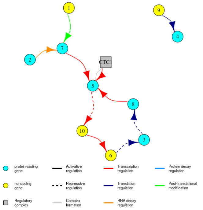
For small networks, you can try to use plotGRN(mysystem, plotType = "interactive2D") to get dynamic 2D plots. Note that you can pass additional arguments to plotGRN that will be used by the plot.igraph function from the igraph package to plot the network (see https://igraph.org/r/doc/plot.common.html for the list of available arguments). This can be useful for example if your network is large, because the arrows will look too big and you won’t be able to see much. To correct that you can use plotGRN(mysystem, edge.arrow.size = 0.5).

The edge dataframe shows the global GRN, with all the different types of regulations. The element mosystem of the insilicosystem object contains the same edges but grouped by type of regulation:

> names(mysystem$mosystem)

[1] "TCRN_edg"  "TLRN_edg"  "RDRN_edg"  "PDRN_edg"  "PTMRN_edg"

> mysystem$mosystem$TCRN_edg

  from to TargetReaction RegSign RegBy TCbindingrate TCunbindingrate TCfoldchange
1    5 10             TC      -1    PC  1.261302e-06    0.0004756718     0.000000
2    7  5             TC       1    PC  5.004492e-07    0.0011372389     7.133808
3    8  5             TC       1    PC  1.035420e-07    0.0012070782    10.859677
4 CTC1  5             TC       1     C  4.001311e-06    0.0014327934     5.809262
5   10  6             TC       1    NC  1.436779e-04    0.0018526967    12.131921

Here you can only see the edges of the GRN corresponding to the regulation of transcription. Each of the sub-GRNs stored in the mosystem element contains additional information about the kinetic parameters associated with each edge. For example, we can see that each edge corresponding to a regulatory interaction targeting the transcription is assigned a binding rate (TCbindingrate) and an unbinding rate (TCunbindingrate) of the regulator to and from the binding site on the target gene’s promoter. The parameter TCfoldchange corresponds to the coefficient by which is multiplied the basal transcription rate of the target when the regulator is bound to its binding site (for edges for which RegSign = "-1", i.e. corresponding to a repression, the fold change TCfoldchange is automatically set to 0, e.g. row 1). The kinetic parameters associated with each edge depend on the type of regulation:

> lapply(mysystem$mosystem, function(x){colnames(x)[-(1:5)]})

$TCRN_edg
[1] "TCbindingrate"   "TCunbindingrate" "TCfoldchange"   

$TLRN_edg
[1] "TLbindingrate"   "TLunbindingrate" "TLfoldchange"   

$RDRN_edg
[1] "RDregrate"

$PDRN_edg
[1] "PDregrate"

$PTMRN_edg
[1] "PTMregrate"

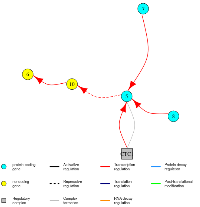
Again, it is possible to visualise these subnetworks: the function plotGRN can restrict the type of edges displayed to a specific type of regulation. For example to only see edges in the GRN corresponding to regulation of transcription, you can use:

plotGRN(mysystem, "TC")

plotGRNTC

The regulatory complexes

In the GRN, some regulations can be performed by regulatory complexes. The composition of these complexes is stored in the complexes element of the insilicosystem object.

> mysystem$complexes

$CTC1
[1] "5" "5"

This means that 2 of the products of gene 5 assemble in the system to form a regulatory complex labelled “CTC1”. Note that the complex does not have to be formed by the products of a single gene, but can be composed of the products of different genes. The kinetic parameters associated with these complexes (i.e. association and dissociation rates of the components) are available with:

> mysystem$complexeskinetics

$CTC1
$CTC1$formationrate
[1] 0.001583534

$CTC1$dissociationrate
[1] 87.55631

The element complexesTargetReaction of the insilicosystem object simply gives the type of regulation that the complexes accomplish, here regulation of transcription:

> mysystem$complexesTargetReaction

$CTC1
[1] "TC"

The `sysargs` element

The different parameters used to generate the in silico system are stored in the sysargs element of the insilicosystem object. You can specify a value for each of these parameters during the construction of the system, by passing them to the function generateInSilicoSystem. The list of all parameters is shown in Appendix.

Modifying the in silico system

It is possible to modify your system. In particular, you can:

Add a gene:

> mysystem2 = addGene(mysystem)
> mysystem2$genes

   id coding TargetReaction PTMform ActiveForm       TCrate     TLrate       RDrate       PDrate
 1     NC            PTM       0         R1 0.0022650092 0.00000000 0.0006022248 0.000000e+00
 2     PC             RD       0         P2 0.0011610575 1.45493135 0.0012704290 5.241792e-04
 3     PC             TL       0         P3 0.0008440692 0.07610997 0.0005346026 4.659461e-04
 4     PC             MR       0         P4 0.0018660167 0.02094220 0.0005450206 9.495481e-05
 5     PC             TC       0         P5 0.0013195158 0.08482105 0.0015738163 3.724944e-04
 6     NC             TL       0         R6 0.0017867835 0.00000000 0.0009361317 0.000000e+00
 7     PC             TC       1        Pm7 0.0050424625 0.08673830 0.0003888850 9.668181e-04
 8     PC             TC       0         P8 0.0040488925 0.52078680 0.0008828149 2.566280e-04
 9     NC             TL       0         R9 0.0008180618 0.00000000 0.0007097201 0.000000e+00
10     NC             TC       0        R10 0.0034226576 0.00000000 0.0003839845 0.000000e+00
11     PC             TL       0        P11 0.0010205586 0.06387881 0.0014847265 6.886111e-04

Notice that the function does not modify the mysystem system but creates a new insilicosystem object. Here we simply asked for a new gene to be created, and the function chooses whether it is protein-coding or noncoding and samples its kinetic parameters. Alternatively we can specify these different arguments:

> mysystem2 = addGene(mysystem, coding = "PC", TargetReaction = "TL", TCrate = 0.005, PDrate = 0.0007)
> mysystem2$genes

   id coding TargetReaction PTMform ActiveForm       TCrate     TLrate       RDrate       PDrate
 1     NC            PTM       0         R1 0.0022650092 0.00000000 0.0006022248 0.000000e+00
 2     PC             RD       0         P2 0.0011610575 1.45493135 0.0012704290 5.241792e-04
 3     PC             TL       0         P3 0.0008440692 0.07610997 0.0005346026 4.659461e-04
 4     PC             MR       0         P4 0.0018660167 0.02094220 0.0005450206 9.495481e-05
 5     PC             TC       0         P5 0.0013195158 0.08482105 0.0015738163 3.724944e-04
 6     NC             TL       0         R6 0.0017867835 0.00000000 0.0009361317 0.000000e+00
 7     PC             TC       1        Pm7 0.0050424625 0.08673830 0.0003888850 9.668181e-04
 8     PC             TC       0         P8 0.0040488925 0.52078680 0.0008828149 2.566280e-04
 9     NC             TL       0         R9 0.0008180618 0.00000000 0.0007097201 0.000000e+00
10     NC             TC       0        R10 0.0034226576 0.00000000 0.0003839845 0.000000e+00
11     PC             TL       0        P11 0.0050000000 0.02279752 0.0008311582 7.000000e-04

There is for now no way to remove a gene from an existing in silico system (for computational reasons).

Add or remove an edge in the GRN:

If we want gene 3, a regulator of translation, to activate the expression (translation) of gene 5, we can use:

> mysystem2 = addEdge(mysystem, regID = 1, tarID = 5, regsign = "1",
                       kinetics = list("TCbindingrate" = 0.01,
                                       "TCunbindingrate" = 0.1,
                                       "TCfoldchange" = 10))

> tail(mysystem$edg) ## Original system

   from to TargetReaction RegSign RegBy
5    10  6             TC       1    NC
6     6  3             TL      -1    NC
7     9  4             TL       1    NC
8     3  8             TL      -1    PC
9     2  7             RD       1    PC
10    1  7            PTM       1    NC

> tail(mysystem2$edg) ## System with the new edge

   from to TargetReaction RegSign RegBy
6     6  3             TL      -1    NC
7     9  4             TL       1    NC
8     3  8             TL      -1    PC
9     2  7             RD       1    PC
10    1  7            PTM       1    NC
11    3  5             TL       1    PC

> mysystem$mosystem$TLRN_edg ## Original system

  from to TargetReaction RegSign RegBy TLbindingrate TLunbindingrate TLfoldchange
1    6  3             TL      -1    NC  1.666402e-04    0.0006129013     0.000000
2    9  4             TL       1    NC  9.458748e-04    0.0015561749     7.171744
3    3  8             TL      -1    PC  1.784989e-06    0.0008773741     0.000000

> mysystem2$mosystem$TCRN_edg ## System with the new edge

  from to TargetReaction RegSign RegBy TLbindingrate TLunbindingrate TLfoldchange
1    6  3             TL      -1    NC  1.666402e-04    0.0006129013     0.000000
2    9  4             TL       1    NC  9.458748e-04    0.0015561749     7.171744
3    3  8             TL      -1    PC  1.784989e-06    0.0008773741     0.000000
4    3  5             TL       1    PC  1.000000e-02    0.1000000000    10.000000

Note that the kinetic parameters of the regulatory interaction are passed in a named list. If the names of the parameters provided are wrong, the function won’t stop with an error but will instead sample values for the parameters, as it would do if the parameters weren’t provided at all. You cannot choose which expression step of the target is regulated, as it depends on the biological function of the regulator. It must be noted that the regulator can be either a gene or a regulatory complex.

Similarly we can remove the edge, with:

> mysystem2 = removeEdge(mysystem2, regID = 3, tarID = 5)
> mysystem2$mosystem$TLRN_edg

  from to TargetReaction RegSign RegBy TLbindingrate TLunbindingrate TLfoldchange
1    6  3             TL      -1    NC  1.666402e-04    0.0006129013     0.000000
2    9  4             TL       1    NC  9.458748e-04    0.0015561749     7.171744
3    3  8             TL      -1    PC  1.784989e-06    0.0008773741     0.000000

Add or remove a regulatory complex:

We can create new regulatory complexes, by choosing the genes whose products will associate:

> mysystem2 = addComplex(mysystem, compo = c(6, 9))
> mysystem2$complexes

$CTC1
[1] "5" "5"

$CTL1
[1] "6" "9"

The created complex is named CTL1. Again, you can specify the association and dissociation rate of the complex by passing the arguments formationrate and dissociationrate to the function. The components of the new complex must have the same biological function:

> mysystem2 = addComplex(mysystem, compo = c(6, 7))

Error in addComplex(mysystem, compo = c(6, 7)) : 
  The different components do not all have the same biological function.

We can remove a regulatory complex from a system. By doing so, all edges coming from the complex will be removed from the system:

> mysystem2 = removeComplex(mysystem, "CTC1")
> mysystem2$complexes

named list()

> mysystem$mosystem$TCRN_edg ## Original system

  from to TargetReaction RegSign RegBy TCbindingrate TCunbindingrate TCfoldchange
1    5 10             TC      -1    PC  1.261302e-06    0.0004756718     0.000000
2    7  5             TC       1    PC  5.004492e-07    0.0011372389     7.133808
3    8  5             TC       1    PC  1.035420e-07    0.0012070782    10.859677
4 CTC1  5             TC       1     C  4.001311e-06    0.0014327934     5.809262
5   10  6             TC       1    NC  1.436779e-04    0.0018526967    12.131921

> mysystem2$mosystem$TCRN_edg ## System without the complex

  from to TargetReaction RegSign RegBy TCbindingrate TCunbindingrate TCfoldchange
1    5 10             TC      -1    PC  1.261302e-06    0.0004756718     0.000000
2    7  5             TC       1    PC  5.004492e-07    0.0011372389     7.133808
3    8  5             TC       1    PC  1.035420e-07    0.0012070782    10.859677
4   10  6             TC       1    NC  1.436779e-04    0.0018526967    12.131921

Empty in silico system

The argument "empty" of the generateInSilicoSystem function allows you to generate a system without any regulatory interactions:

> emptysystem = createInSilicoSystem(G = 7, empty = T)
> emptysystem$edg

[1] from           to             TargetReaction RegSign        RegBy         
<0 rows> (or 0-length row.names)

Creating an in silico population

We will next create a population of in silico individuals. Each individual possesses one or more copies of the genes specified in the in silico system (generated in the previous step), as specified by the ploidy of the system. You can decide the number of different alleles of each gene that exist in this in silico population, etc. For example:

mypop = createInSilicoPopulation(3, mysystem, ngenevariants = 4)

creates a population of 3 in silico diploid individuals (ploidy = 2 specified in the previous section), assuming that there exist 4 different (genetically speaking) alleles of each gene. The population returned by the function is an object of class insilicopopulation, i.e. a list whose different attributes are presented below.

The gene alleles

A gene allele is represented as a vector containing the quantitative effects of its mutations on different kinetic properties of the gene, termed QTL effect coefficients. The alleles existing in this population are stored in the element GenesVariants of the insilicopopulation object returned by the function.

> mypop$GenesVariants[1:2]

$`1`
              1         2         3        4
qtlTCrate     1 1.0000000 1.0000000 1.000000
qtlRDrate     1 0.9522776 1.0000000 1.000000
qtlTCregbind  1 1.0000000 0.9762780 1.007287
qtlRDregrate  1 1.0000000 0.9910411 1.000000
qtlactivity   1 1.0374314 1.0000000 1.000000
qtlTLrate     0 0.0000000 0.0000000 0.000000
qtlPDrate     0 0.0000000 0.0000000 0.000000
qtlTLregbind  0 0.0000000 0.0000000 0.000000
qtlPDregrate  0 0.0000000 0.0000000 0.000000
qtlPTMregrate 0 0.0000000 0.0000000 0.000000

$`2`
              1         2         3         4
qtlTCrate     1 1.0000000 0.9400730 1.0000000
qtlRDrate     1 1.0000000 1.0375015 1.0073818
qtlTCregbind  1 1.0000000 1.0000000 1.1013731
qtlRDregrate  1 1.0000000 0.8505525 0.8238966
qtlactivity   1 1.0000000 1.2285846 1.0303434
qtlTLrate     1 0.9419998 1.1578962 0.9689810
qtlPDrate     1 1.0000000 0.9321794 0.9710529
qtlTLregbind  1 1.0000000 1.0481206 1.2379087
qtlPDregrate  1 1.0000000 0.7584668 1.2236113
qtlPTMregrate 1 1.0000000 0.8749443 1.1218343

This shows the alleles (columns of the dataframe) of genes 1 and 2 that have been generated by the function. The first allele of each gene corresponds to the “original” version of the gene, i.e. all QTL effect coefficients are set to 1. A QTL effect coefficient is a multiplicative coefficient that will be applied to the corresponding kinetic parameter of the gene during the construction of the stochastic model to simulate the expression profiles for the different individuals. As some of the QTL effect coefficients apply to translation- or protein-related steps of the gene expression, they are set to 0 for noncoding genes (see gene 1).

Here, the 4th allele of gene 1 carries two mutations (two QTL effect coefficient different from 1). The first mutation decreases the RNA decay rate of the gene (qtlRDrate < 1). The second mutation increases the activity of the gene’s active product (qtlactivity > 1). Gene 1 being a noncoding gene (coding = "NC") encoding a regulatory RNA controlling the post-transcriptional modification of its targets (TargetReaction = "PTM"), it means that the RNAs of this variant will modify its target proteins with an increased rate compared to the original version of the gene.

QTL effect coefficient name	Effect
`qtlTCrate`	Affects the basal transcription rate of the gene
`qtlRDrate`	Affects the basal RNA decay rate of the gene
`qtlTCregbind`	Affects the binding rate of the regulators of transcription on the gene’s promoter (affects all transcription regulators targeting this gene)
`qtlRDregrate`	Affects the rate at which regulators of RNA decay encountering the RNAs of the gene trigger their degradation (affects all RNA decay regulators targeting this gene)
`qtlactivity`	Affects the activity of the active product of the gene. If the gene is encoding for a regulator of transcription or translation, this affects the binding rate of its active products (i.e. RNAs or proteins) to their binding sites on their targets (affects the binding to all targets of the gene). If the gene encodes a regulator of RNA or protein decay or of protein post-translational modification, this affects the rate at which its active products (i.e. RNAs or proteins) trigger the degradation/transformation of their targets (effect for all targets of the gene).
`qtlTLrate`	Affects the basal translation rate of the gene
`qtlPDrate`	Affects the basal protein decay rate of the gene
`qtlTLregbind`	Affects the binding rate of the regulators of translation on the gene’s RNA binding sites (affects all translation regulators targeting this gene)
`qtlPDregrate`	Affects the rate at which regulators of protein decay encountering the proteins of the gene trigger their degradation (affects all protein decay regulators targeting this gene)
`qtlPTMregrate`	Affects the rate at which regulators of protein post-translational modification encountering the proteins of the gene trigger their modification (affects all protein post-translational modification regulators targeting this gene)

The in silico individuals

The different generated in silico individuals are stored in the element individualsList of the insilicopopulation object. Each individual is represented by a list with the following elements:

haplotype: gives for each gene (rows) the alleles that the individual carries (columns). The different copies of the genes are denoted “GCNi”, (with i ranging from 1 to P - the ploidy of the organism). In this example we defined the ploidy of the system to be 2, so each individual carries 2 copies of each gene.
```
> mypop$individualsList$Ind1$haplotype

 GCN1 GCN2
1     3    2
2     1    1
3     2    2
4     3    2
5     3    3
6     1    1
7     3    1
8     2    3
9     1    4
10    1    4
```
Here the first individual (Ind1) carries two copies of allele 3 of gene 5, and the alleles 2 and 3 of gene 1.
QTLeffects: gives for each gene copy (i.e. “GCN1”, “GCN2”, etc) the value of each QTL effect coefficient for the genes (value for gene i at the i-th position in the vector of QTL effect coefficients).

> mypop$individualsList$Ind1$QTLeffects$GCN1

$qtlTCrate
 [1] 1.0000000 1.0000000 0.9672539 0.9383817 1.0000000 1.0000000 1.0000000 1.0812009 1.0000000 1.0000000

$qtlRDrate
 [1] 1.0000000 1.0000000 1.0000000 0.9346013 0.9554500 1.0000000 0.9614498 1.0000000 1.0000000 1.0000000

$qtlTCregbind
 [1] 0.9762780 1.0000000 0.9209159 1.0512399 1.0000000 1.0000000 0.9259654 1.0000000 1.0000000 1.0000000

$qtlRDregrate
 [1] 0.9910411 1.0000000 0.9275185 1.0000000 1.1410932 1.0000000 1.0000000 1.0706625 1.0000000 1.0000000

$qtlactivity
 [1] 1.0000000 1.0000000 1.0000000 1.1118578 1.0620914 1.0000000 0.9806165 1.0000000 1.0000000 1.0000000

$qtlTLrate
 [1] 0.0000000 1.0000000 1.0498663 1.0000000 0.9686472 0.0000000 1.0000000 1.0000000 0.0000000 0.0000000

$qtlPDrate
 [1] 0.0000000 1.0000000 1.1117630 1.0000000 1.0144363 0.0000000 0.7340314 1.0850892 0.0000000 0.0000000

$qtlTLregbind
 [1] 0.0000000 1.0000000 1.1650171 0.9199958 1.1522007 0.0000000 0.9378752 0.9753078 0.0000000 0.0000000

$qtlPDregrate
 [1] 0.0000000 1.0000000 0.8805382 1.0000000 1.0000000 0.0000000 1.0000000 1.0000000 0.0000000 0.0000000

$qtlPTMregrate
 [1] 0.0000000 1.0000000 0.9818818 1.0799951 1.0000000 0.0000000 1.0000000 1.0811174 0.0000000 0.0000000
 

As individual Ind1’s first copy (“GCN1”) of gene 2 is gene 2’s allele 1 (see mypop$GenesVariants[[2]][,1]), the 2nd element of each QTL effect coefficient vector for GCN1 is 1.0. Similarly, the 3rd element of the different QTL effect coefficients vectors for GCN1 correspond to the values in mypop$GenesVariants[[3]][,2] (as the first Ind1’s copy of gene 3 is gene 3’s allele 2).

InitAbundance: the list of initial abundance for the RNAs and proteins of the genes. During the simulation of the individuals gene profiles, a stochastic system is generated and an initial abundance is required for each product (RNA and protein) of the different genes. This initial abundance is automatically computed during the construction of each in silico individual, and corresponds to the steady-state abundance of the molecule in absence of any regulation (i.e. production rate / decay rate) accounting for the effects of the genetic mutations. When constructing the in silico population, the parameter initialNoise controls whether or not these initial abundances are exactly equal to their no-regulation steady state abundance. If not (default behaviour of the createInSilicoPopulation function), the initial abundance of a given molecule is instead sampled from a normal distribution with a mean equal to this no-regulation steady state abundance, and a standard deviation equal to the square root of the aforementioned steady-state abundance. Note that the square root of the mean is used as standard deviation to reduce the variation for molecules with low abundance. The initial abundances of an individual are stored in a list that separates the different copies of each gene (here GCN1 and GCN2), and the RNA and protein forms of the genes (R and P). The initial abundance for gene i is given at the i-th position of the vectors:

> mypop$individualsList$Ind1$InitAbundance

$GCN1
$GCN1$R
 [1]  1  1  1  5  1  1 17  3  1  8

$GCN1$P
 [1]    0 2489  217  732  174    0 1708 9393    0    0


$GCN2
$GCN2$R
 [1]  2  1  2  3  3  3 15  3  2  5

$GCN2$P
 [1]    0 2561  257  761  199    0 1174 9527    0    0

For example for Ind1, there are initially 1 molecule of the RNA form of gene 1’s first copy (GCN1) in the system, while there are 2 molecules of gene 1’s second copy (GCN2). The proteins of both copies of gene 10 are initially not present in the system (initial abundance both at 0), which is logical since gene 10 is noncoding, and thus does not produce proteins.

It is possible to visualise the QTL effect coefficients of all the genes in the system for each in silico individual in the population, with:

plotMutations(mypop, mysystem, nGenesPerRow = 5)

plotMutations

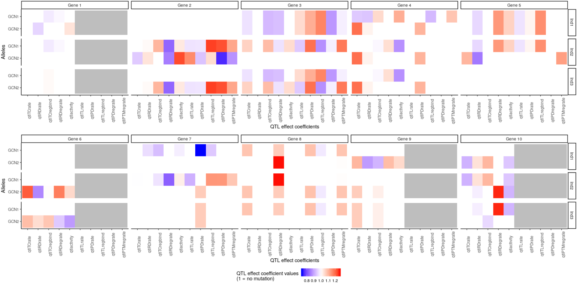
The function plotMutations takes as arguments the in silico population and the in silico system, and plot the value (colour) of each QTL effect coefficient (x-axis) for each copy (y-axis) of each gene (columns) for each individual in the population (rows). (The argument nGenesPerRow simply indicates how many genes to plot per row in the final plot, useful when the number of genes is large to avoid plots that are too wide).

As we saw with the haplotype element, we can see that the first individual Ind1 carries two identical copies of gene 5, because the values of the QTL effect coefficients are identical in both copies. However individual Ind3 carries two different alleles of gene 3 (the values of the QTL effect coefficients are different for the two copies GCN1 and GCN2).

The second copy (GCN2) of gene 3 for individual Ind2 is the original version of the gene, i.e. the QTL effect coefficients all have a value of 1 (white) meaning that this version does not have any mutation. Notice that genes 1, 6, 9 and 10 are nocoding genes. Consequently, the QTL effect coefficients related to protein or translation are not applicable, and they are represented in gray.

You can of course focus the plot on only some individuals, genes, gene copy, QTL effect coefficients or even values, with the arguments passed to plotMutations, as in:

plotMutations(mypop, mysystem,
              scaleLims = c(0.85, 1.15),
              qtlEffectCoeffs = c("qtlTCrate", "qtlTLrate", "qtlRDrate", "qtlPDrate"),
              inds = c("Ind1", "Ind2"),
              alleles = "GCN2",
              genes = 1:3)

plotMutations2

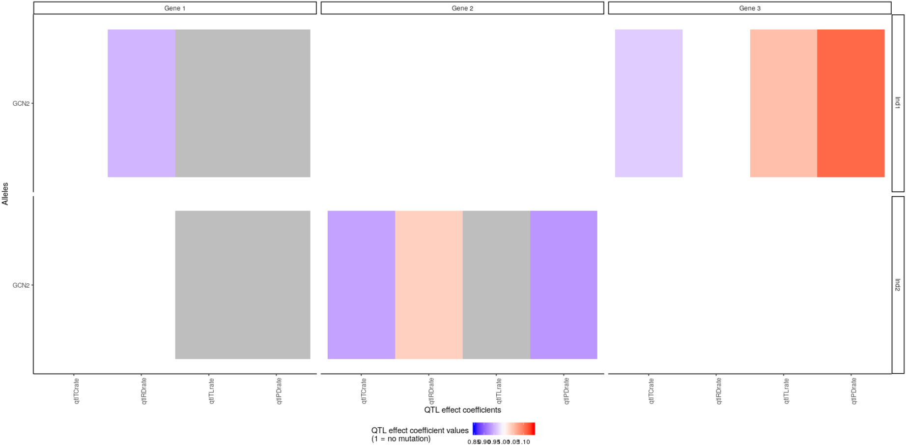
Here we restricted the plot to the second allele of genes 1, 2, and 3 for the first two individuals. We only represented the QTL effect coefficients affecting the basal kinetic properties of the gene (transcription, translation, RNA decay and protein decay rate). We also restricted the plot to QTL effect coefficients whose values were between 0.85 and 1.15. This is why the qtlTLrate value of gene 2 for Ind2 is in gray: not because it is are not applicable but because its values range outside these limits:

> mypop$individualsList$Ind2$QTLeffects$GCN2$qtlTLrate[2]
[1] 1.157896

The `indargs` element

The different parameters used to generate the in silico individuals are stored in the indargs element of the insilicopopulation object. You can specify a value for each of these parameters during the construction of the system, by passing them to the function generateInSilicoPopulation. The list of all parameters is shown in Appendix.

Simulating the system

Once the system and the population have been defined, we can simulate the expression of the genes in the system for each in silico individual. We use the function:

sim = simulateInSilicoSystem(mysystem, mypop, simtime = 2000, ntrials = 5)

simtime allows you to control the simulation end time in seconds (here we simulate the expression of the genes for 2000s). ntrials correspond to the number of repetitions of the simulation that will be computed for each individual (here set to 5). To speed-up the running time, Linux and MacOS users can use a parallelised version of the simulation function:

sim = simulateParallelInSilicoSystem(mysystem, mypop, simtime = 2000, ntrials = 5)

The output of the simulation is a list of 3 elements. The element runningtime gives the elapsed time between the beginning and the end of the simulations (all repetitions) for each individual.

> sim$runningtime

[1] 71.754 42.657 63.007

If you used the parallelised function simulateParallelInSilicoSystem, then sim$runningtime only gives the running time of the entire set of simulations (i.e. for all repetitions of all individuals).

The stochmodel element returned as an output of the simulation is a XRJulia proxy object giving Julia object that stores the stochastic model of the system (do not try to read it, it is not really useful in its current form - rather, see the The stochastic model section).

The result of the simulation, that is the abundance of the different species in the system over time for each in silico individual, is returned in the Simulation element. This is a data-frame, giving for each individual (column Ind), for each repetition of the simulation (column trial) the abundance of the different species over time (column time).

> head(sim$Simulation)

  time trial R5GCN2 P5GCN2 R7GCN2 P7GCN2 Pm7GCN2 R3GCN1 P3GCN1 R1GCN2 R9GCN1 R6GCN2 R10GCN2 R1GCN1 R4GCN2 P4GCN2 R8GCN1 P8GCN1 R6GCN1
  0     1      3    199     15   1174       0      1    217      2      1      3       5      1      3    761      3   9393      1
  1     1      3    194     15   1172       0      1    217      2      1      3       5      1      3    761      3   9389      1
  2     1      3    196     15   1173       0      1    216      2      1      3       5      1      3    761      3   9386      1
  3     1      3    199     15   1175       0      1    216      2      1      3       5      1      3    762      3   9378      1
  4     1      3    198     15   1174       0      1    216      2      1      3       5      1      3    763      3   9376      1
  5     1      3    198     15   1173       0      1    217      2      1      3       5      1      3    764      3   9379      1
  R10GCN1 R2GCN2 P2GCN2 R8GCN2 P8GCN2 R5GCN1 P5GCN1 R4GCN1 P4GCN1 R3GCN2 P3GCN2 R2GCN1 P2GCN1 R9GCN2 R7GCN1 P7GCN1 Pm7GCN1
     8      1   2561      3   9527      1    174      5    732      2    257      1   2489      2     17   1708       0
     8      1   2560      3   9525      1    171      5    732      2    257      1   2494      2     17   1711       0
     8      1   2559      3   9522      1    173      5    732      2    257      1   2495      2     17   1711       0
     8      1   2559      3   9523      1    172      5    732      2    258      1   2496      2     15   1715       0
     8      1   2560      3   9522      1    173      5    731      2    258      1   2497      2     15   1716       0
     8      1   2564      3   9519      1    171      5    731      2    258      1   2496      2     14   1718       0
  CTC1_P5GCN1_P5GCN1 CTC1_P5GCN2_P5GCN2 CTC1_P5GCN1_P5GCN2 CTC1_P5GCN2_P5GCN1  Ind
                0                  0                  0                  0 Ind1
                0                  1                  1                  2 Ind1
                0                  1                  0                  1 Ind1
                1                  0                  0                  0 Ind1
                0                  0                  1                  0 Ind1
                1                  0                  0                  1 Ind1

By default, the simulation distinguishes the different gene products (RNAs, proteins and regulatory complexes) according to their copy of origin (e.g. the RNAs arising from the first and second copy of gene 1 will be separately counted in the columns R1GCN1 and R1GCN2, respectively). To obtain results that ignore the copy of origin, you can use:

> simNoAllele = mergeAlleleAbundance(sim$Simulation)
> head(simNoAllele)

  time trial  Ind R5  P5 R7   P7 Pm7 R3  P3 R1 R9 R6 R10 R4   P4 R8    P8 R2   P2 CTC1_P5_P5
1    0     1 Ind1  4 373 32 2882   0  3 474  3  3  4  13  8 1493  6 18920  2 5050          0
2    1     1 Ind1  4 365 32 2883   0  3 474  3  3  4  13  8 1493  6 18914  2 5054          4
3    2     1 Ind1  4 369 32 2884   0  3 473  3  3  4  13  8 1493  6 18908  2 5054          2
4    3     1 Ind1  4 371 30 2890   0  3 474  3  3  4  13  8 1494  6 18901  2 5055          1
5    4     1 Ind1  4 371 30 2890   0  3 474  3  3  4  13  8 1494  6 18898  2 5057          1
6    5     1 Ind1  4 369 29 2891   0  3 475  3  3  4  13  8 1495  6 18898  2 5060          2

A gene product bound into a regulatory complex is not accounted for when computing the abundance for this species (e.g. if all existing proteins of gene 5 are in a regulatory complex then the abundance for P5 will be 0). It is possible to ignore the regulatory complexes and compute the abundance of a species by counting each molecule whether it is in a free form or bound into a complex:

> simNoComplex = mergeComplexesAbundance(sim$Simulation)
> head(simNoComplex)

  time trial R5GCN2 P5GCN2 R7GCN2 P7GCN2 Pm7GCN2 R3GCN1 P3GCN1 R1GCN2 R9GCN1 R6GCN2 R10GCN2 R1GCN1 R4GCN2 P4GCN2 R8GCN1 P8GCN1 R6GCN1
  0     1      3    199     15   1174       0      1    217      2      1      3       5      1      3    761      3   9393      1
  1     1      3    199     15   1172       0      1    217      2      1      3       5      1      3    761      3   9389      1
  2     1      3    199     15   1173       0      1    216      2      1      3       5      1      3    761      3   9386      1
  3     1      3    199     15   1175       0      1    216      2      1      3       5      1      3    762      3   9378      1
  4     1      3    199     15   1174       0      1    216      2      1      3       5      1      3    763      3   9376      1
  5     1      3    199     15   1173       0      1    217      2      1      3       5      1      3    764      3   9379      1
  R10GCN1 R2GCN2 P2GCN2 R8GCN2 P8GCN2 R5GCN1 P5GCN1 R4GCN1 P4GCN1 R3GCN2 P3GCN2 R2GCN1 P2GCN1 R9GCN2 R7GCN1 P7GCN1 Pm7GCN1  Ind
     8      1   2561      3   9527      1    174      5    732      2    257      1   2489      2     17   1708       0 Ind1
     8      1   2560      3   9525      1    174      5    732      2    257      1   2494      2     17   1711       0 Ind1
     8      1   2559      3   9522      1    174      5    732      2    257      1   2495      2     17   1711       0 Ind1
     8      1   2559      3   9523      1    174      5    732      2    258      1   2496      2     15   1715       0 Ind1
     8      1   2560      3   9522      1    174      5    731      2    258      1   2497      2     15   1716       0 Ind1
     8      1   2564      3   9519      1    174      5    731      2    258      1   2496      2     14   1718       0 Ind1

Lastly, non-modified and (post-translationally) modified forms of proteins are counted separately. We merge their abundance with:

> simNoPTM = mergePTMAbundance(simNoAllele)
> head(simNoPTM)

  time trial  Ind R5  P5 R7   P7 R3  P3 R1 R9 R6 R10 R4   P4 R8    P8 R2   P2 CTC1_P5_P5
1    0     1 Ind1  4 373 32 2882  3 474  3  3  4  13  8 1493  6 18920  2 5050          0
2    1     1 Ind1  4 365 32 2883  3 474  3  3  4  13  8 1493  6 18914  2 5054          4
3    2     1 Ind1  4 369 32 2884  3 473  3  3  4  13  8 1493  6 18908  2 5054          2
4    3     1 Ind1  4 371 30 2890  3 474  3  3  4  13  8 1494  6 18901  2 5055          1
5    4     1 Ind1  4 371 30 2890  3 474  3  3  4  13  8 1494  6 18898  2 5057          1
6    5     1 Ind1  4 369 29 2891  3 475  3  3  4  13  8 1495  6 18898  2 5060          2

All merging functions presented above require a dataframe as imput. They can be used one after the other or independently, e.g.:

> simNothing = mergeComplexesAbundance(simNoAllele)
> head(simNothing)

  time trial  Ind R5  P5 R7   P7 Pm7 R3  P3 R1 R9 R6 R10 R4   P4 R8    P8 R2   P2
1    0     1 Ind1  4 373 32 2882   0  3 474  3  3  4  13  8 1493  6 18920  2 5050
2    1     1 Ind1  4 373 32 2883   0  3 474  3  3  4  13  8 1493  6 18914  2 5054
3    2     1 Ind1  4 373 32 2884   0  3 473  3  3  4  13  8 1493  6 18908  2 5054
4    3     1 Ind1  4 373 30 2890   0  3 474  3  3  4  13  8 1494  6 18901  2 5055
5    4     1 Ind1  4 373 30 2890   0  3 474  3  3  4  13  8 1494  6 18898  2 5057
6    5     1 Ind1  4 373 29 2891   0  3 475  3  3  4  13  8 1495  6 18898  2 5060

Plotting the simulation

It is possible to visualise the results of the simulation with:

plotSimulation(sim$Simulation)

plotSimulation

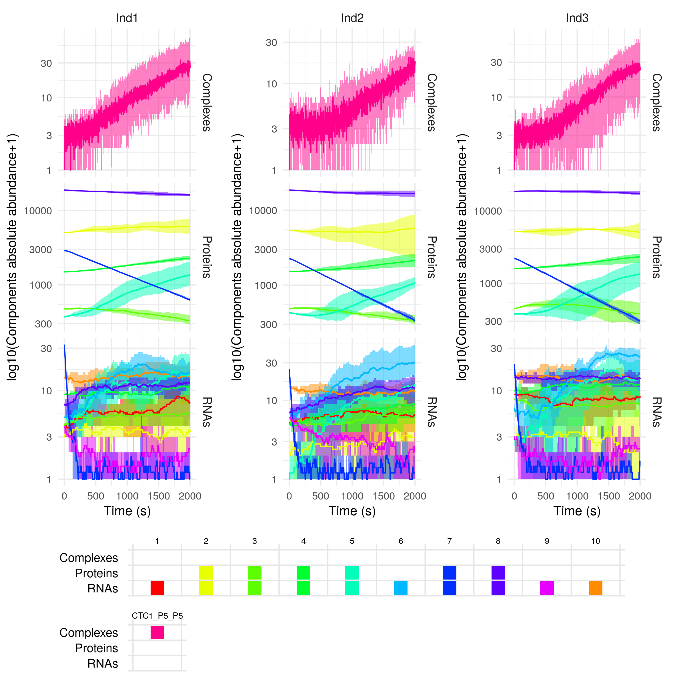
This returns a plot of the abundance of the different species (separated by RNAs -bottom-, proteins -middle- and regulatory complexes -top-) over time. As the simulation has been repeated 5 times for each individual(ntrials = 5), the mean abundance over the different repetitions or trials of the molecules is plotted as a solid line, and the minimum and maximum values are represented by the coloured areas. By default the abundances are plotted on a log10 scale, but you can change that with the option yLogScale = F in the plotSimulation function.

By default, the different gene copies are merged before plotting (mergeAllele = T), and similarly the non-modified and modified versions of the proteins are merged before plotting (mergePTM = T). On the contrary, the free and in complex components of the system are not merged (mergeComplexes = F).

The legend is presented as a table that gives for each component (columns) the different forms it can be found in. For example if we decide not to merge the non-modified and modified versions of the proteins, we have:

plotSimulation(sim$Simulation, mergePTM = F)

plotSimulationPTM

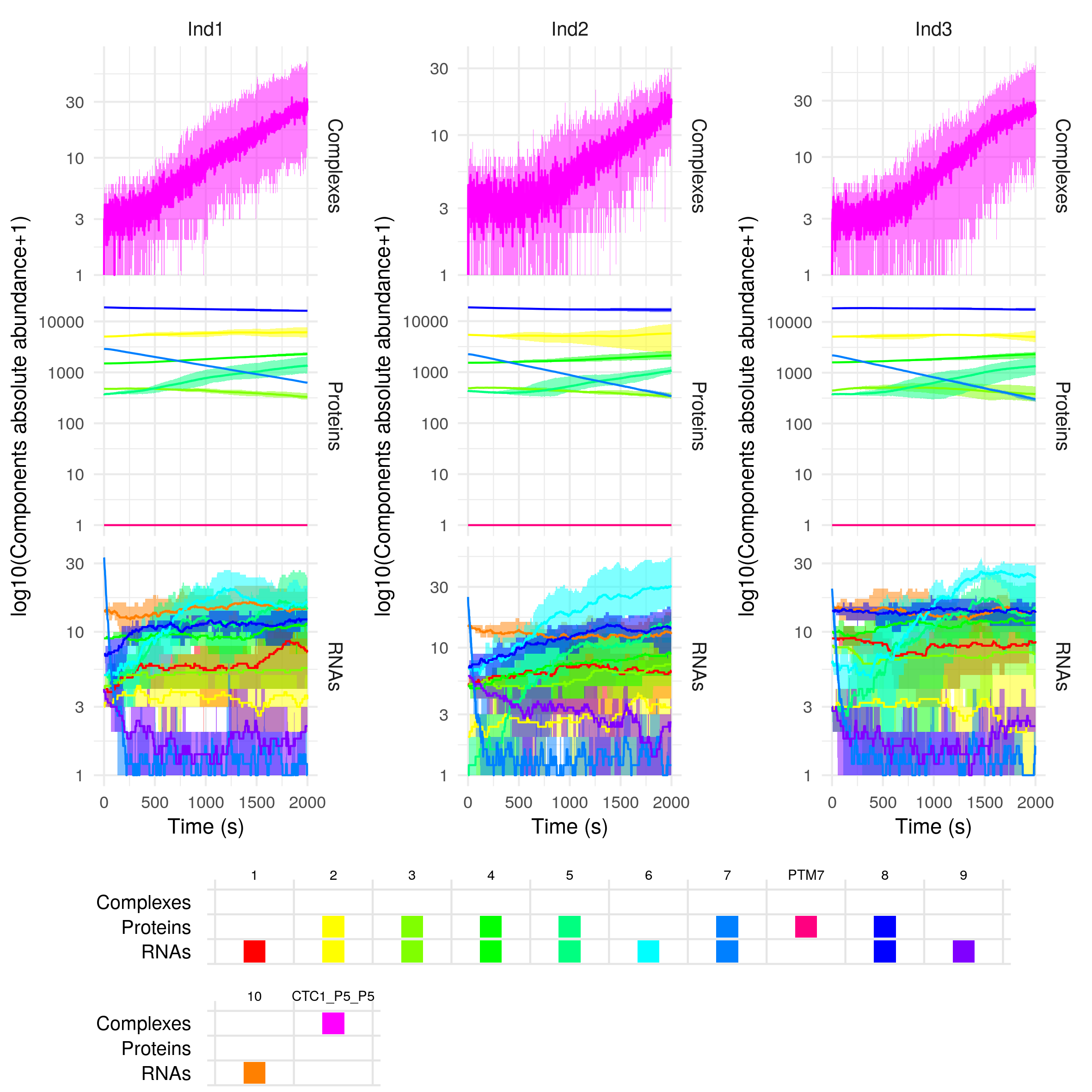
The first component names are numbers, they correspond to the gene IDs. We can find the different genes either as RNAs or proteins if they are protein-coding (e.g. gene 1), or only as RNAs if the genes are noncoding (e.g. gene 2). As gene 7 is targeted for post-translational modification, there exists a modified form of its protein, PTM7. The component CTC1 is a regulatory complex. Its full name, CTL1_P5_P5 contains the list of its constituents, here two proteins of gene 5.

To help you get an idea of the general tendencies of the abundance of the different components, the function summariseSimulation returns a dataframe giving for each component (row) and each individual (column) the maximum and final average abundance over the different trials:

> sumtable = summariseSimulation(sim$Simulation)
--------------------------
Summary of simulation for:
--------------------------
Individuals: Ind1 Ind2 Ind3 
Trials: 1 2 3 4 5 
Time: 0 s - 2000 s
--------------------------

> head(sumtable)

  Components Abundance   Ind1   Ind2   Ind3
1         R1       Max    7.6    6.4    8.2
2         R1     Final    6.2    5.6    7.6
3         R2       Max    3.2    3.4    2.4
4         R2     Final    2.4    2.4    1.2
5         P2       Max 6129.8 5767.0 5578.6
6         P2     Final 6127.6 5767.0 5063.2

The function prints on your console the individuals, trials and timespan considered for the summary. You can suppress this display with the argument verbose = F in the function call.

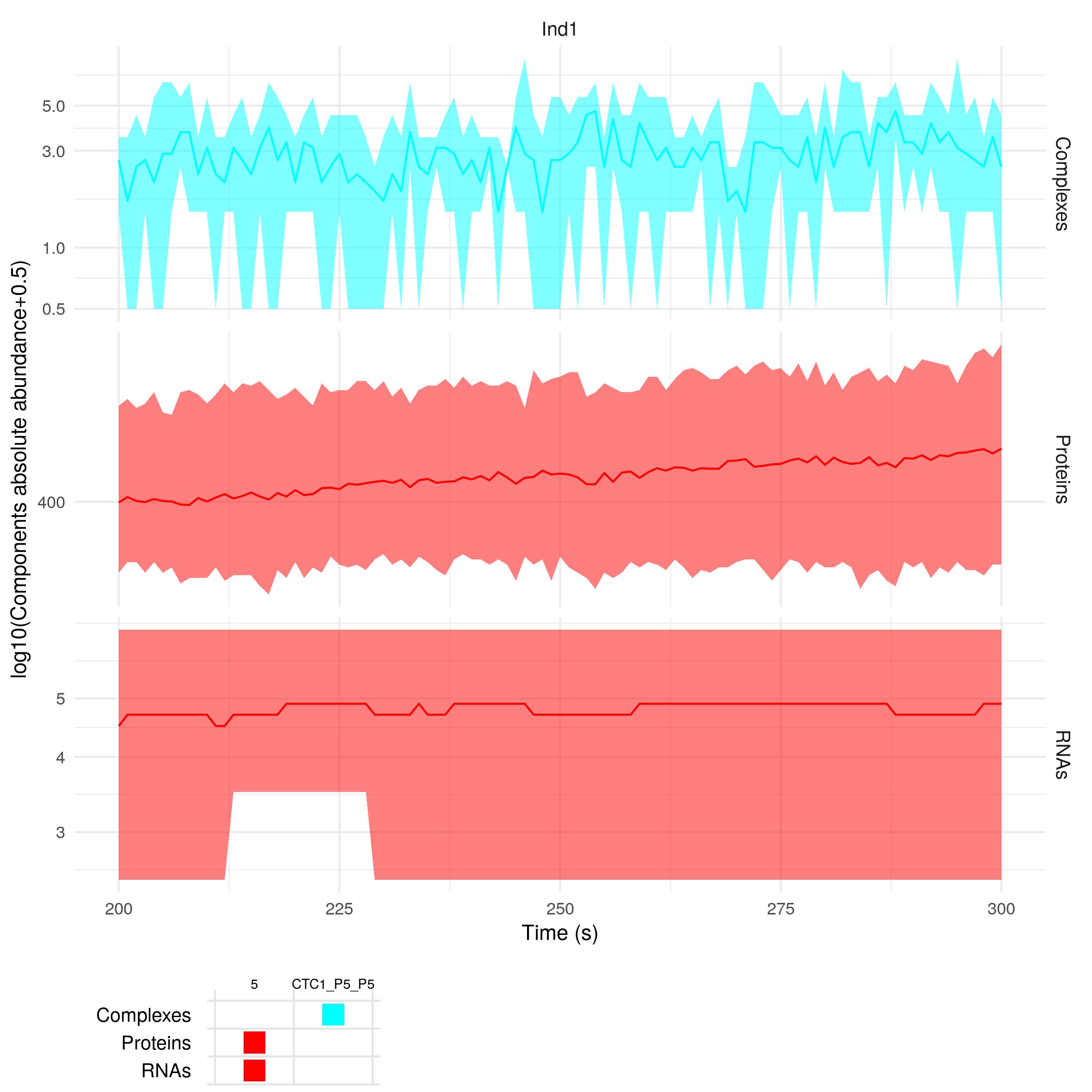
If you want to focus on one in silico individual, a specific group of genes, and zoom on a smaller time-period, you can use:

plotSimulation(sim$Simulation, molecules = c(5, "CTC1"), inds = c("Ind1"), timeMin = 200, timeMax = 300)

plotSimulation2

The function summariseSimulation takes as input the same arguments as the function plotSimulation, so you can also do:

> sumtable = summariseSimulation(sim$Simulation, inds = c("Ind1"), timeMin = 200, timeMax = 300)
--------------------------
Summary of simulation for:
--------------------------
Individuals: Ind1 
Trials: 1 2 3 4 5 
Time: 200 s - 300 s
--------------------------

> head(sumtable)

  Components Abundance   Ind1
1         R1       Max    4.2
2         R1     Final    4.2
3         R2       Max    2.8
4         R2     Final    2.6
5         P2       Max 5322.0
6         P2     Final 5322.0

Alernatively, you can plot the abundance of the different components as a heatmap:

plotHeatMap(sim$Simulation)

plotHeatMap

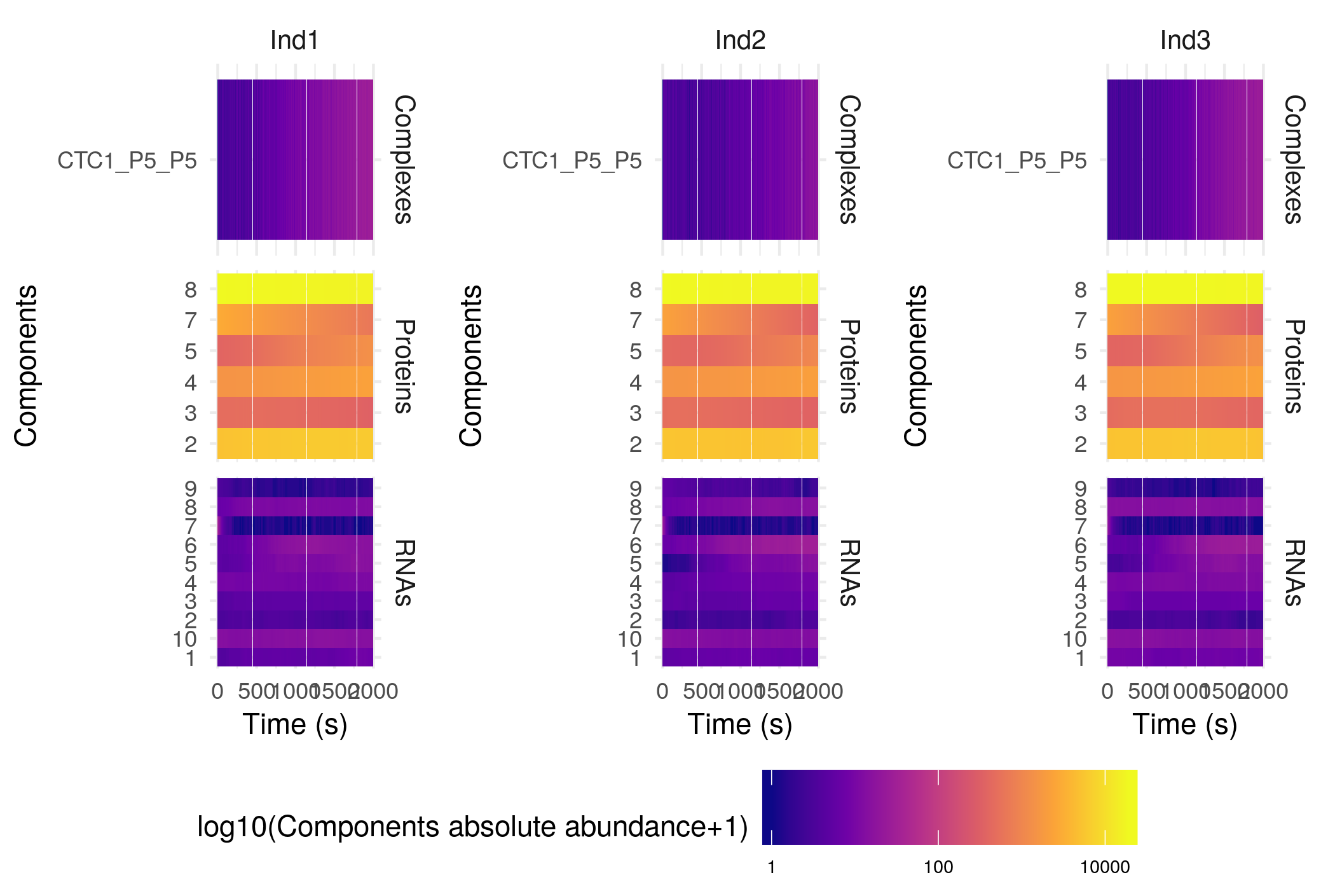
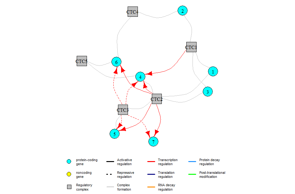
The settings of this function are the same as those of the plotSimulation function presented above. Plotting this specific simulation as a heatmap is not really useful, but such plot can get really interesting for more complex cases, as for example the anthocyanin biosynthesis regulation pathway (included as an example here): plotcolpw

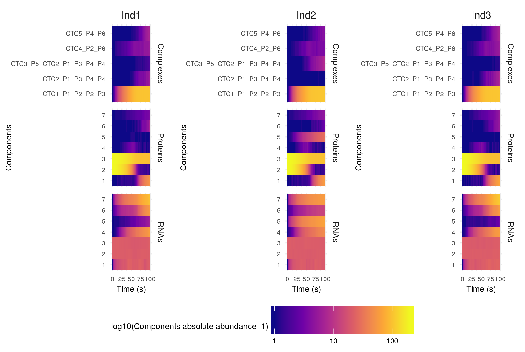
The GRN for this example is:

plotGRNcolpw

Note that both plotSimulation and plotHeatMap can take as input additional parameters that will be passed to ggplot2::theme() when plotting the simulation (see https://ggplot2.tidyverse.org/reference/theme.html for the list of available parameters). This is useful for example if your axis titles are too small or too large (or if you want them in red).

The stochastic model

If you want to see the list of species and reactions (i.e. the stochastic model) of the system, you can use the option writefile = T and specify the directory in which the files text files will be saved (argument filepath) of the simulate(Parallel)inSilicoSystem functions. Note that if you omit to specify the output directory (filepath), the writefile argument will be ignored. This generates two text files: one listing the different species in the system, each line giving the name of a species and its initial abundance, and one listing the biochemical reactions and associated rates. The initial abundances and reaction rates are written in a general form (i.e. giving the QTL effect coefficients/initial abundance variation coefficients to be used to compute numerical values for each individual). The species and reactions files for this in silico system are available (here)[https://github.com/oliviaAB/sismonr/tree/master/docs/example/].

The species

As the individuals are diploid, there exist two versions of each gene (and gene product): the one originating from the first copy (GCN1) and the one originating from the second copy (GCN2), e.g.:

R1GCN1

R1GCN2

The DNA sequence of genes is not explicitely modelled, except if the gene is regulated at the transcription level. In this case, the gene’s DNA form is modelled as the sum of its binding sites for its different regulators. These binding sites can exist in a free or bound state. Morevoer, the binding site of a specific regulator can be occupied by the regulator’s product arising from either of the regulator copies. For example, gene 10 transcription is regulated by gene 5, so the DNA form of gene 10’s first allele is:

Pr10GCN1reg5F 1 ## free binding site for regulator 5 on gene 10’s first copy

Pr10GCN1reg5GCN1B 0 ## binding site occupied by one of regulator 5’s products originating from the first copy of the gene

Pr10GCN1reg5GCN2B 0 ## binding site occupied by one of regulator 5’s products originating from the second copy of the gene

The same scheme is repeated for the second copy of gene 10:

Pr10GCN2reg5F 1

Pr10GCN2reg5GCN1B 0

Pr10GCN2reg5GCN2B 0

At the beginning of the simulation, all binding sites are in a free state (initial abundance 1 for the free form of the binding sites, 0 for the occupied forms).

The same modelling applies to the RNA form of genes. If the gene is not targeted by regulators of translation (e.g. gene 1), we simply have:

R1GCN1 InitAbundance[“GCN1”][“R”][1]

R1GCN2 InitAbundance[“GCN2”][“R”][1]

The initial abundance of gene 1’s RNAs is specified in the InitAbundance element of each individual. If on the contrary the gene is targeted by regulators of translation, the RNA form of the gene is modelled as the sum of the RNA binding sites for the different translation regulators. One example is gene 3 whose translation is regulated by gene 6:

RBS3GCN1reg6F InitAbundance[“GCN1”][“R”][3]

RBS3GCN1reg6GCN1B 0

RBS3GCN1reg6GCN2B 0

RBS3GCN2reg6F InitAbundance[“GCN2”][“R”][3]

RBS3GCN2reg6GCN1B 0

RBS3GCN2reg6GCN2B 0

Again, at the beginning of the simulation, all RNA binding sites are in a free state.

The proteins are modelled as follow:

P2GCN1 InitAbundance[“GCN1”][“P”][2]

P2GCN2 InitAbundance[“GCN2”][“P”][2]

If a gene is targeted in the GRN by post-translational modification, there also exists a modified form of the protein, e.g. for gene 7:

P7GCN1 InitAbundance[“GCN1”][“P”][7]

P7GCN2 InitAbundance[“GCN2”][“P”][7]

Pm7GCN1 0

Pm7GCN2 0

At the beginning of the simulation all proteins are in their original (non-modified) form.

Recall that in our system, two molecules of gene 5’s product assemble into a regulatory complex named CTC1. As there exist two versions of the proteins of this gene (arising either from the first or the second copy of the gene), there exist 4 versions of the complex, including all possible combinations of the different protein versions (here we could reduce it to 2 versions as the complex is a homodimer, but that would not be possible if the complex was formed by the products of two different genes). Initially no regulatory complex is formed in the system.

CTC1_P5GCN1_P5GCN1 0

CTC1_P5GCN1_P5GCN2 0

CTC1_P5GCN2_P5GCN1 0

CTC1_P5GCN2_P5GCN2 0

The reactions

Each reaction is characterised by a name, a biochemical formula in the form “$\sum$ reactants $\rightarrow$ $\sum$ products”, and a rate. For example the formation and dissociation of the regulatory complex CTL1 are (from the section above we know that there are 4 versions of the complex, hence 8 formation/dissociation reactions):

formationCTC1_P5GCN1_P5GCN1 P5GCN1 + P5GCN1 –> CTC1_P5GCN1_P5GCN1 0.00158353441270883

dissociationCTC1_P5GCN1_P5GCN1 CTC1_P5GCN1_P5GCN1 –> P5GCN1 + P5GCN1 87.5563075786515

formationCTC1_P5GCN1_P5GCN2 P5GCN1 + P5GCN2 –> CTC1_P5GCN1_P5GCN2 0.00158353441270883

dissociationCTC1_P5GCN1_P5GCN2 CTC1_P5GCN1_P5GCN2 –> P5GCN1 + P5GCN2 87.5563075786515

formationCTC1_P5GCN2_P5GCN1 P5GCN2 + P5GCN1 –> CTC1_P5GCN2_P5GCN1 0.00158353441270883

dissociationCTC1_P5GCN2_P5GCN1 CTC1_P5GCN2_P5GCN1 –> P5GCN2 + P5GCN1 87.5563075786515

formationCTC1_P5GCN2_P5GCN2 P5GCN2 + P5GCN2 –> CTC1_P5GCN2_P5GCN2 0.00158353441270883

dissociationCTC1_P5GCN2_P5GCN2 CTC1_P5GCN2_P5GCN2 –> P5GCN2 + P5GCN2 87.5563075786515

Generating RNA-seq-like data

sismonr now includes a function to transform a given time-point of a simulation into RNA-seq-like data, i.e. returns for each RNA molecule a simulated read count for each individual, with the function:

rnaseqData = getRNAseqMatrix(sim$Simulation, mysystem, samplingTime = 500, mrnasOnly = T)

Each individual is considered as a separate sample in the RNA-seq experiment. The parameter samplingTime indicates which time-point to transform. If no value is provided, the function will use the last time-point in the simulation. The parameter mrnasOnly determines whether non-coding RNAs will be included in the transformation. By default mrnasOnly = T, and thus only protein-coding RNAs are considered. The generation of RNA-seq-like data works as follow:

For each individual, the absolute abundance of the different (protein-coding) RNAs are transformed into (noisy) proportions. In an RNA-seq experiment, not all RNA molecules are extracted from the samples, and thus it is possible that the proportions of mRNAs of each gene into the sample to be processed may not be exactly equal to the true mRNA proportions. In particular, some mRNAs present with very low abundance may not be detected. To reproduce this bias, only a fraction of all the RNA molecules in the system is sampled. The user can control this fraction with the parameter propRnasSampled. Setting propRnasSampled to 1 corresponds to transforming the absolute abundance of the RNAs into their exact proportion in the system, while setting the parameter to a value lower than 1 introduces some noise in the proportions.
For each individual, the proportions of the different RNAs are multiplied by the corresponding gene length. This step reproduces the bias of RNA-seq experiments in which longer genes create more reads. By default, sismonr assigns to each gene a length of 1. However, the user can provide a length for each gene through the parameter genesLength. The proportions are then re-scaled so that their sum over all genes in each individual is 1.
An expected library size is sampled for each individual. Again, the user can provide the expected library size of each individual/sample with the parameter samplesLibSize. Otherwise, expected library sizes are sampled from a log-normal distribution with mean meanLogLibSize_lane (default value of 7, giving a mean expected library size of $10^7$) and a standard deviation of sdLogLibSize_samples. sismonr is also able to simulate a batch effect in the library size: in an RNA-seq experiment, processing the samples on different lanes can affect their resulting library size, as some lanes may generate more or less reads than the others. Thus setting the parameter laneEffect allows to simulate the processing of the individuals on different lanes (number of lanes controlled by the parameter nLanes). In this case, a mean log-library size is first sampled for each lane from a normal distribution with meanmeanLogLibSize_lane and standard deviation sdLogLibSize_lane. Then each individual is randomnly assigned to a lane, and its expected library size is sampled from a log-normal distribution with mean equal to the sampled mean log-library size of the corresponding lane and standard deviation sdLogLibSize_samples.
The expected read count of RNA in each individual is obtained by multiplying the proportion of the RNA by the expected library size of the individual.
Read counts for each RNA in each individual are sampled from a Poisson distribution with parameter equal to the expected count of the corresponding RNA in the corresponding sample.

The object returned by the function getRNAseqMatrix() is a list, containing the following information:

rnaSeqMatrix: a dataframe giving for each gene (rows) the simulated read counts in each individual (columns).

> rnaseqData$rnaSeqMatrix

# A tibble: 6 x 4
  Molecule    Ind1    Ind2    Ind3
  <chr>      <int>   <int>   <int>
1 R2        611976  880457  415953
2 R3       1220530 2494283  996548
3 R4       2442344 3224400 1865675
4 R5       2576783 1760480  788334
5 R7         67980  146641       0
6 R8       2986943 6012220 2281935

samplesLibSize: a list providing the lane on which each sample was “processed” (element lane), the expected library size of each sample (element expected_library_size), and the mean library size for each lane (element lane_mean_library_size). If the individuals expected library sizes were provided by the user, only the element expected_library_size is returned.

> rnaseqData$samplesLibSize

$lane
Ind1 Ind2 Ind3 
   1    1    1 

$expected_library_size
    Ind1     Ind2     Ind3 
 9905311 14517683  6346089 

$lane_mean_library_size
    1 
1e+07 

genesLength: the length of each gene.

> rnaseqData$genesLength

2 3 4 5 7 8 
1 1 1 1 1 1 

Appendix

Parameters for in silico system generation

This is the list of all the parameters that can be passed to the createInSilicoSystem function when generating an in silico system, that control the different properties of the system.

G: Integer. Number of genes in the system. Default value is 10.
ploidy: Integer. Number of copy for each gene that the in silico individuals carry (ploidy of the system). Default value is 2.
PC.p: Numeric. Probability of each gene to be a protein-coding gene. Default value is 0.7.
PC.TC.p: Numeric. Probability of a protein-coding gene to be a regulator of transcription. Default value is 0.4.
PC.TL.p: Numeric. Probability of a protein-coding gene to be a regulator of translation. Default value is 0.3.
PC.RD.p: Numeric. Probability of a protein-coding gene to be a regulator of RNA decay. Default value is 0.1.
PC.PD.p: Numeric. Probability of a protein-coding gene to be a regulator of protein decay. Default value is 0.1.
PC.PTM.p: Numeric. Probability of a protein-coding gene to be a regulator of protein post-translational modification. Default value is 0.05.
PC.MR.p: Numeric. Probability of a protein-coding gene to be a metabolic enzyme. Default value is 0.05.
NC.TC.p: Numeric. Probability of a noncoding gene to be a regulator of transcription. Default value is 0.3.
NC.TL.p: Numeric. Probability of a noncoding gene to be a regulator of translation. Default value is 0.3.
NC.RD.p: Numeric. Probability of a noncoding gene to be a regulator of RNA decay. Default value is 0.3.
NC.PD.p: Numeric. Probability of a noncoding gene to be a regulator of protein decay. Default value is 0.05.
NC.PTM.p: Numeric. Probability of a noncoding gene to be a regulator of protein post-translational modification. Default value is 0.05.
TC.pos.p: Numeric. Probability of a regulation targeting gene transcription to be positive. Default value is 0.5.
TL.pos.p: Numeric. Probability of a regulation targeting gene translation to be positive. Default value is 0.5.
PTM.pos.p: Numeric. Probability of a regulation targeting protein post-translational modification to be positive (i.e the targeted protein is transformed into its modified form, as opposed to the modified protein being transformed back into its original form). Default value is 0.5.
basal_transcription_rate_samplingfct: Function from which the transcription rates of genes are sampled (input x is the required sample size). Default value is a function returning $(10^v)/3600$, with $v$ a vector of size x sampled from a normal distribution with mean of 3 and sd of 0.5.
basal_translation_rate_samplingfct: Function from which the translation rates of genes are sampled (input x is the required sample size). Default value is a function returning $(10^v)/3600$, with $v$ a vector of size x sampled from a normal distribution with mean of 2.146 and sd of 0.7.
basal_RNAlifetime_samplingfct: Function from which the transcript lifetimes are sampled (input x is the required sample size). Default value is a function returning $(10^v)*3600$, with $v$ a vector of size x sampled from a normal distribution with mean of 0.95 and sd of 0.2.
basal_protlifetime_samplingfct: Function from which the protein lifetime are sampled (input x is the required sample size). Default value is a function returning $(10^v)*3600$, with $v$ a vector of size x sampled from a normal distribution with mean of 1.3 and sd of 0.4.
TC.PC.outdeg.distr: Form of the distribution of the number of targets (out-degree) of protein regulators in the transcription regulation graph; can be either “powerlaw” or “exponential”. Default value is “powerlaw”.
TC.NC.outdeg.distr: Form of the distribution of the number of targets (out-degree) of noncoding regulators in the transcription regulation graph; can be either “powerlaw” or “exponential”. Default value is “powerlaw”.
TC.PC.outdeg.exp: Numeric. Exponent of the distribution for the out-degree of the protein regulators in the transcription regulation graph. Default value is 3.
TC.NC.outdeg.exp: Numeric. Exponent of the distribution for the out-degree of the noncoding regulators in the transcription regulation graph. Default value is 5.
TC.PC.indeg.distr: Type of preferential attachment for the targets of protein regulators in the transcription regulation graph; can be either “powerlaw” or “exponential”. Default value is “powerlaw”.
TC.NC.indeg.distr: Type of preferential attachment for the targets of noncoding regulators in the transcription regulation graph; can be either “powerlaw” or “exponential”. Default value is “powerlaw”.
TC.PC.autoregproba: Numeric. Probability of protein regulators to perform autoregulation in the transcription regulation graph. Default value is 0.2.
TC.NC.autoregproba: Numeric. Probability of noncoding regulators to perform autoregulation in the transcription regulation graph. Default value is 0.
TC.PC.twonodesloop: Logical. Are 2-nodes loops authorised in the transcription regulation graph with protein regulators? Default value is FALSE.
TC.NC.twonodesloop: Logical. Are 2-nodes loops authorised in the transcription regulation graph with noncoding regulators? Default value is FALSE.
TCbindingrate_samplingfct: Function from which the binding rates of transcription regulators on their targets are sampled (input means is a vector of length equal to the required sample size, giving for each edge (regulatory interaction) for which a binding rate is being sampled the value of the sampled unbinding rate divided by the steady-state abundance of the regulator in absence of any regulation in the system). Default value is a function returning $10^v$, where $v$ is a vector with the same length as means whose elements are sampled from a truncated normal distribution with mean equal to the log10 of the corresponding element in means, and sd = 0.1, the minimum authorised value being the log10 of the corresponding element in means.
TCunbindingrate_samplingfct: Function from which the unbinding rates of transcription regulators from their target are sampled (input x is the required sample size). Default value is a function returning $10^v$, with $v$ a vector of size x sampled from a normal distribution with mean of -3 and sd of 0.2.
TCfoldchange_samplingfct: Function from which the transcription fold change induced by a bound regulator is sampled (input x is the required sample size). Default value is a truncated normal distribution with a mean of 3, sd of 10 and minimum authorised value of 1.5.
TL.PC.outdeg.distr: Form of the distribution of the number of targets (out-degree) of protein regulators in the translation regulation graph; can be either “powerlaw” or “exponential”. Default value is “powerlaw”.
TL.NC.outdeg.distr: Form of the the distribution of the number of targets (out-degree) of noncoding regulators in the translation regulation graph; can be either “powerlaw” or “exponential”. Default value is “powerlaw”.
TL.PC.outdeg.exp: Numeric. Exponent of the distribution for the out-degree of the protein regulators in the translation regulation graph. Default value is 4.
TL.NC.outdeg.exp: Numeric. Exponent of the distribution for the out-degree of the noncoding regulators in the translation regulation graph. Default value is 6.
TL.PC.indeg.distr: Type of preferential attachment for the targets of protein regulators in the translation regulation graph; can be either “powerlaw” or “exponential”. Default value is “powerlaw”.
TL.NC.indeg.distr: Type of preferential attachment for the targets of noncoding regulators in the translation regulation graph; can be either “powerlaw” or “exponential”. Default value is “powerlaw”.
TL.PC.autoregproba: Numeric. Probability of protein regulators to perform autoregulation in the translation regulation graph. Default value is 0.2.
TL.NC.autoregproba: Numeric. Probability of noncoding regulators to perform autoregulation in the translation regulation graph. Default value is 0.
TL.PC.twonodesloop: Logical. Are 2-nodes loops authorised in the translation regulation graph with protein regulators? Default value is FALSE.
TL.NC.twonodesloop: Logical. Are 2-nodes loops authorised in the translation regulation graph with noncoding regulators? Default value is FALSE.
TLbindingrate_samplingfct: Function from which the binding rate of translation regulators on target are sampled (input means is a vector of length equal to the required sample size, giving for each edge (regulatory interaction) for which a binding rate is being sampled the value of the sampled unbinding rate divided by the steady-state abundance of the regulator in absence of any regulation in the system). Default value is a function returning $10^v$, where $v$ is a vector with the same length as means whose elements are sampled from a truncated normal distribution with mean equal to the log10 of the corresponding element in means, and sd = 0.1, the minimum authorised value being the log10 of the corresponding element in means.
TLunbindingrate_samplingfct: Function from which the unbinding rate of translation regulators from target are sampled (input x is the required sample size). Default value is a function returning $10^v$, with $v$ a vector of size x sampled from a normal distribution with mean of -3 and sd of 0.2.
TLfoldchange_samplingfct: Function from which the translation fold change induced by a bound regulator are sampled (input x is the required sample size). Default value is a truncated normal distribution with a mean of 3, sd of 10 and minimum authorised value of 1.5.
RD.PC.outdeg.distr: Form of the distribution of the number of targets (out-degree) of protein regulators in the RNA decay regulation graph; can be either “powerlaw” or “exponential”. Default value is “powerlaw”.
RD.NC.outdeg.distr: Form of the the distribution of the number of targets (out-degree) of noncoding regulators in the RNA decay regulation graph; can be either “powerlaw” or “exponential”. Default value is “powerlaw”.
RD.PC.outdeg.exp: Numeric. Exponent of the distribution for the out-degree of the protein regulators in the RNA decay regulation graph. Default value is 4.
RD.NC.outdeg.exp: Numeric. Exponent of the distribution for the out-degree of the noncoding regulators in the RNA decay regulation graph. Default value is 6.
RD.PC.indeg.distr: Type of preferential attachment for the targets of protein regulators in the RNA decay graph; can be either “powerlaw” or “exponential”. Default value is “powerlaw”.
RD.NC.indeg.distr: Type of preferential attachment for the targets of noncoding regulators in the RNA decay graph; can be either “powerlaw” or “exponential”. Default value is “powerlaw”.
RD.PC.autoregproba: Numeric. Probability of protein regulators to perform autoregulation in the RNA decay regulation graph. Default value is 0.2.
RD.NC.autoregproba: Numeric. Probability of noncoding regulators to perform autoregulation in the RNA decay regulation graph. Default value is 0.
RD.PC.twonodesloop: Logical. Are 2-nodes loops authorised in the RNA decay regulation graph with protein regulators? Default value is FALSE.
RD.NC.twonodesloop: Logical. Are 2-nodes loops authorised in the RNA decay regulation graph with noncoding regulators? Default value is FALSE.
RDregrate_samplingfct: Function from which the RNA decay rates of targets of RNA decay regulators are sampled (input x is the required sample size). Default value is a function returning $10^v$, with $v$ a vector of size x sampled from a normal distribution with mean of -5 and sd of 1.5.
PD.PC.outdeg.distr: Form of the distribution of the number of targets (out-degree) of protein regulators in the protein decay regulation graph; can be either “powerlaw” or “exponential”. Default value is “powerlaw”.
PD.NC.outdeg.distr: Form of the the distribution of the number of targets (out-degree) of noncoding regulators in the protein decay regulation graph; can be either “powerlaw” or “exponential”. Default value is “powerlaw”.
PD.PC.outdeg.exp: Numeric. Exponent of the distribution for the out-degree of the protein regulators in the protein decay regulation graph. Default value is 4.
PD.NC.outdeg.exp: Numeric. Exponent of the distribution for the out-degree of the noncoding regulators in the protein decay regulation graph. Default value is 6.
PD.PC.indeg.distr: Type of preferential attachment for the targets of protein regulators in the protein decay regulation graph; can be either “powerlaw” or “exponential”. Default value is “powerlaw”.
PD.NC.indeg.distr: Type of preferential attachment for the targets of noncoding regulators in the protein decay graph; can be either “powerlaw” or “exponential”. Default value is “powerlaw”.
PD.PC.autoregproba: Numeric. Probability of protein regulators to perform autoregulation in the protein decay regulation graph. Default value is 0.2.
PD.NC.autoregproba: Numeric. Probability of noncoding regulators to perform autoregulation in the protein decay regulation graph. Default value is 0.
PD.PC.twonodesloop: Logical. Are 2-nodes loops authorised in the protein decay graph with protein regulators in the protein decay regulation graph? Default value is FALSE.
PD.NC.twonodesloop: Logical. Are 2-nodes loops authorised in the protein decay graph with noncoding regulators in the protein decay regulation graph? Default value is FALSE.
PDregrate_samplingfct: Function from which the protein decay rates of targets of protein decay regulators are sampled (input x is the required sample size). Default value is a function returning $10^v$, with $v$ a vector of size x sampled from a normal distribution with mean of -5 and sd of 1.5.
PTM.PC.outdeg.distr: Form of the distribution of the number of targets (out-degree) of protein regulators in the post-translational modification regulation graph; can be either “powerlaw” or “exponential”. Default value is “powerlaw”.
PTM.NC.outdeg.distr: Form of the the distribution of the number of targets (out-degree) of noncoding regulators in the post-translational modification regulation graph; can be either “powerlaw” or “exponential”. Default value is “powerlaw”.
PTM.PC.outdeg.exp: Numeric. Exponent of the distribution for the out-degree of the protein regulators in the protein post-translational modification graph. Default value is 4.
PTM.NC.outdeg.exp: Numeric. Exponent of the distribution for the out-degree of the noncoding regulators in the protein post-translational modification graph. Default value is 6.
PTM.PC.indeg.distr: Type of preferential attachment for the targets of protein regulators in the protein post-translational modification graph; can be either “powerlaw” or “exponential”. Default value is “powerlaw”.
PTM.NC.indeg.distr: Type of preferential attachment for the targets of noncoding regulators in the protein post-translational modification graph; can be either “powerlaw” or “exponential”. Default value is “powerlaw”.
PTM.PC.autoregproba: Numeric. Probability of protein regulators to perform autoregulation. Default value is 0.2.
PTM.NC.autoregproba: Numeric. Probability of noncoding regulators to perform autoregulation. Default value is 0.
PTM.PC.twonodesloop: Logical. Are 2-nodes loops authorised in the protein post-translational modification graph with protein regulators? Default value is FALSE.
PTM.NC.twonodesloop: Logical. Are 2-nodes loops authorised in the protein post-translational modification graph with noncoding regulators? Default value is FALSE.
PTMregrate_samplingfct: Function from which the protein transformation rates of targets of post-translational modification regulators are sampled (input x is the required sample size). Default value is a function returning $10^v$, with $v$ a vector of size x sampled from a normal distribution with mean of -5 and sd of 1.5.
regcomplexes: Can the regulators controlling a common target form regulatory complexes in the different regulatory graphs? Can be ‘none’, ‘prot’ (only protein can form regulatory complexes) or ‘both’ (both regulatory RNAs and proteins can form regulatory complexes). Default value is “prot”.
regcomplexes.p: Numeric. Probability that regulators controlling a common target form regulatory complexes; ignore if $regcomplexes$ = ‘none’. Default value is 0.3.
regcomplexes.size: Integer. Number of components of a regulatory complex; ignore if regcomplexes = ‘none’. Default value is 2.
complexesformationrate_samplingfct: Function from which the formation rate of regulatory complexes are sampled (input x is the required sample size). Default value is a function returning $10^v$, with $v$ a vector of size x sampled from a normal distribution with mean of -3 and sd of 0.7.
complexesdissociationrate_samplingfct: Function from which the dissociation rate of regulatory complexes are sampled (input x is the required sample size). Default value is a function returning $10^v$, with $v$ a vector of size x sampled from a normal distribution with mean of 3 and sd of 0.9.

Parameters for in silico individuals generation

This is the list of all the parameters that can be passed to the createInSilicoPopulation function when generating an in silico population, that control the different properties of the individuals.

ngenevariants: Integer. Number of alleles existing for each gene in the in silico population. Default value is 5.
qtleffect_samplingfct: Function from which is sampled the value of a QTL effect coefficient (input x is the required sample size). Default value is a truncated normal distribution with mean 1 and sd 0.1 (only gives positive values).
initvar_samplingfct: Function from which is sampled the variation of the initial abundance of a species (input x is the required sample size). Default value is a truncated normal distribution with mean 1 and sd 0.1 (only gives positive values).